Time Series Forecasting: Error Metrics to Evaluate Model Performance
8 Forecast error metrics you should know to evaluate the accuracy of your time series models. Find metrics that are aligned with your business goals.
Introduction
The idea of this post comes from the different error metrics I have dealt with working with time series data and forecasting models.
Among other things, we make energy production forecasts of renewable power plants of different capacities and technologies. Our aim is to develop forecasting models that reduce the penalties caused by the deviations.
Most of the models I work with are regression models, and therefore in this article I am focusing only on regression error metrics.
Unfortunately, there is no absolute “right” accuracy metric. Choosing the right metric is a problem-specific matter, and it involves answering questions like:
- Which decision will you base on the forecast?
- What are the consequences of a wrong forecast?
- Who is going to check and monitorize the errors?
- Do we care about the percentage error or about the magnitude of the deviation?
- Does it makes any difference to over-forecast or under-forecast the variable of interest?
Answering the above questions lead us to determine we need to find a metric that:
- Is scale independent, so the errors are comparable between power plants.
- Is symmetric, as we do not want to weight the deviations differently according to their sign.
- Express the error in absolute terms, so the error reflects the real-life imbalance costs.
- The error calculated over different periods should be equivalent to the aggregated calculation over those periods individually.
Each metric behaves in a certain way and therefore reflects in a unique manner the features of the models. Depending on their properties, we can classify the metrics in several categories. Let’s take a look at them:
Scale dependent error metrics
Maybe the most popular and simple error metric is MAE:
MAE:
The Mean Absolute Error is defined as:
\[ MAE = \frac{1}{N}\sum_{t=1}^{N} |A_t - F_t| \]
While the MAE is easily interpretable (each residual contributes proportionally to the total amount of error), one could argue that using the sum of the residuals is not the best choice, as we could want to highlight especially whether the model incur in some large errors.
MSE & RMSE
For those cases, maybe MSE (Mean Squared Error) or RMSE (Root Mean Squared Error) are a better choice. Here the error grows quadratically and therefore extreme values penalize the metric to a greater extent.
\[ MSE = \frac{1}{N} \sum_{t=1}^{N} |A_t - F_t|^2 \]
\[ RMSE = \sqrt{MSE} \]
The main problem with scale dependent metrics is that they are not suitable to compare errors from different sources.
In our case, the capacity of the power plants would determine the magnitude of the errors and therefore comparing them between facilities would not make much sense. This is something we should try to avoid when choosing the metric.
Percentage-error metrics
Next group express the error in percentage terms.
MAPE
The most widespread one is the Mean Absolute Percentage Error:
\[ MAPE_\% = \frac{1}{N}\sum_{t=1}^{N} \frac{|A_t - F_t|}{A_t} \times 100\]
As we said above, depending on our goal, MAPE could be suitable or not. From my point of view percentage error metrics have some major drawbacks. They may give different values for two observations with the same absolute error, depending on whether they share the same actual value or not:
| Case | Actual | Forecast | AbsoluteDifference | MAPE |
|---|---|---|---|---|
| 1 | 100 | 150 | 50 | 50 |
| 2 | 150 | 100 | 50 | 33 |
Besides, MAPE diverges when actual values tend to zero. In our case it is impractical, as this could lead to extreme cases such as:
| Case | Actual | Forecast | AbsoluteDifference | MAPE |
|---|---|---|---|---|
| 3 | 1 | 11 | 10 | 1000 |
That is an undesired behaviour for an error metric since we don’t want to assign huge errors to deviations that involve insignificant operating costs. That suggests a first strong conclusion:
We need to find error metrics that are aligned with our business goals.
Besides, in the example above we can see that MAPE isn’t symmetric as it weights differently two residuals whether the forecast is above or below the actual value. That idea of symmetry lead us to sMAPE.
sMAPE
Trying to solve that assymetry, an alternative to MAPE was proposed. It is called sMAPE, which stands for Symmetric Mean Absolute Percentage Error:
\[ sMAPE_\% = \frac{2}{N} \sum_{t=1}^{N}\frac{|A_t - F_t|}{|A_t| + |F_t|} \times 100\]
However, against all odds Symmetric MAPE is not symmetric: as MAPE, it may present different values for the same absolute deviation:
| Case | Actual | Forecast | AbsoluteDifference | sMAPE |
|---|---|---|---|---|
| 1 | 100 | 150 | 50 | 20 |
| 2 | 100 | 50 | 50 | 33 |
For our use case it is very inconvenient that the same absolute deviation may be quantified with two different error values.
This is a key question: We don’t want to minimize the percentage error but to minimize the economic losses due to forecast deviations, and they are exclusively connected to the sum of the absolute errors. Therefore, we should evaluate the accuracy based on that criteria.
As a final point, simply mention that some others have proposed the Log Ratio \(ln(F_t/A_t)\) as a better alternative to MAPE. You can read a brief description in the previously mentioned sMAPE article or an extended discussion in the original paper by Chris Tofallis
Scale-free error metrics
These are error metrics that have been conveniently normalized to make them dimensionless.
The main advantages of these metrics are:
- Same absolute deviations lead to the same error.
- They are symmetric.
- They are comparable between power plants.
- They are connected to our economic goals.
NMAE
First of all we have NMAE that stands for Normalized Mean Absolute Error. This metric is specific to the energy forecasting business as it is normalized by the capacity C of the power plant, but one could generalize it to any other area provided that there exist an upper bound for the forecasts.
NMAE is expressed as a percentage. It is our preferred metric as it is truly connected with the business goals, it’s easily interpretable and comparable between plants.
\[ NMAE_\% = \frac{1}{N}\sum_{t=1}^{N} \frac{|A_t - F_t|}{C} \times 100\]
Besides, it shows the desirable property:
\[ NMAE_{p1 ∪ p2} = \frac{1}{2}(NMAE_{p1} + NMAE_{p2})\] Given both periods have the same length. If not (e.g: consecutive months), you would only have to adjust by their relative length.
The real-life cost of a forecast error is proportional to the absolute value of the residuals.
The only case when this metric does not apply is whenever the capacity notion has no sense: If the range of the possible values is not bounded, what normalizing constant should I choose?
This would be the case when forecasting temperatures or electricity market prices. Using MAE could be appropiate in these cases, as the units are in the same scale than the magnitude (ºC or €/MWh) and so the errors are easily interpretable, although they would not be truly comparable across different markets or locations.
MAD/Sum Ratio
In energy-related businesses, I have spotted another error metric usually (and, as far as I know, wrongly) called WMAE. Now, WMAE should stand for “Weighted Mean Average Error”. However, the definition I stumbled upon several times was: \[ \frac{1}{N}\frac{ \sum_{t=1}^{N}{|A_t - F_t|}}{\sum_{t=1}^{N}{A_t}} \times 100\]
which is basically the MAE normalized by acummulated energy production.
It resembles MAD/Mean Ratio:
\[ MAD/Mean Ratio_\% = \frac{1}{N}\frac{ \sum_{t=1}^{N}{|A_t - F_t|}}{\frac{1}{N}\sum_{t=1}^{N}{A_t}} \times 100\]
From my point of view, and as an analogy of the MAD/Mean Ratio, the first expression should be called MAD/Sum Ratio. Their properties are similar:
- Their range is [0, \(\infty\)) for non-negative values, which may be difficult to interpret.
- They both show the same asymmetry as MAPE: Different error values come from the same absolute difference between forecasts and actuals.
- Small absolute deviations may be associated to big MAD/Mean or MAD/Sum Ratios, given the actual values are small.
For all those reasons, we insist on the idea that they are kind of disconnected from our loss function.
MASE
There are other scale-free metrics. One of them is MASE (Mean Absolute Scaled Error), proposed by Rob J. Hyndman:
\[ MASE =\frac{\frac{1}{J} \sum_j |A_j - F_j|} {\frac{1}{T-1}\sum_{t=2}^T |A_{t}-A_{t-1}|} \]
where the numerator is the error in the forecast period and the denominator is the MAE of the one-step “naive forecast method” on the training set, that is \(F_t = A_{t-1}\). Because of that, MASE is a metric specifically designed for time series.
Again, whether it is suitable for your needs or not depends entirely on the problem. While it has certain interesting properties such as scale-independence, convergence when \(A_t\to0\) and symmetry, in our case this metric isn’t optimal for several reasons:
- The training series must be completed, i.e., with no gaps. In our case, sometimes we have some measurements missing.
- MASE is equal to 1 when the forecast performance is similar to the naive forecast in the training set. That implies a dependence with the historic period that isn’t always very convenient: if in any given moment we happen to recieve some missing historical production measurements, the accuracy of our model suddenly would change, which may be kind of unintuitive and difficult to track through time.
- MASE is unbounded on the upper side.
- It doesn’t seem to be a friendly metric to use with non-technical people, such as clients or stakeholders: How large are the expected losses for a 1.2 MASE?
EMAE
I found yet another scale-free error metric in a recent paper from the Energy Department of the Politecnico di Milano.
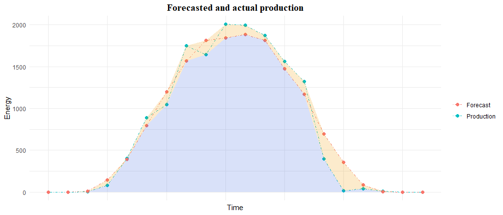
They called it EMAE (Envelope-weighted Mean Absolute Error):
\[ EMAE_\% = \frac{1}{N}\frac{ \sum_{t=1}^{N}{|A_t - F_t|}}{\sum_{t=1}^{N}{\max(A_t, F_t)}} \times 100\]
This metric is quite similar to the MAD/Sum Ratio above but divides by the sum of the maximum between the forecast and the measured power for each observation. It is also expressed as a percentage. This function shows some nice properties:
- It is scale-independent.
- It is symmetric.
- It maps absolute deviation to one unique value.
- It is easily interpretable as its range is [0,100].
- It doesn’t diverge in any point.
- It’s a nice alternative to NMAE since a capacity value is not required.
This formula allows for a cool graphic interpretation of the error: the numerator matchs with the yellow area whereas the denominator corresponds to the sum of the blue and yellow areas:
Conclusions
There is no “best metric” to measure model performance. There are several metrics that highlight different characteristics.
One key aspect is to find error metrics that are connected with our objectives.
Since in most cases the real-life cost of a forecast error is proportional to the absolute value of the residuals, the choice of the metric should be consistent with it.
For our case, NMAE presents the ideal characteristics of interpretability, stability and relation with our loss function that make it the optimal choice.
EMAE is proposed as a nice alternative for the cases NMAE cannot be applied.
References
- Another look at forecast-accuracy metrics for intermittent demand
- Forecasting: Principles and Practice
- Errors on percentage errors
- A new accuracy measure based on bounded relative error for time series forecasting
- Comparison of Training Approaches for Photovoltaic Forecasts by Means of Machine Learning
- On the assymetry of the symmetric MAPE
- A better measure of relative prediction accuracty for model selection and model estimation
- A Guide to Forecast Error Measurement Statistics and How to Use Them
Pablo Cánovas
Senior Data Scientist at Spotahome
Data Scientist, formerly physicist | Tidyverse believer, piping life | Hanging out at TypeThePipe